# 流动性提供：库存、费用与比较基准

重建LP、持币和自融资基准，分离结构LVR、费用层与集中区间状态。

Entry: zh-p33 | Node: P33 | Language: zh | Editorial revision: 2026-09-21

## Teaching instructions
请先实际读取本篇必读原件的指定完整单元，再围绕“重建LP、持币和自融资基准，分离结构LVR、费用层与集中区间状态。”带我完成学习。先让我自己判断方向、对象或基准，再让我逐步重建一项承重计算；不要先把答案全部说出。选读分支只有我选中后才启用对应原件和输入。每次解释都分清真实规则、教学假设、作者报告与本站复算。逐事件核现金、负债、费用和剩余仓位；资金不足时停止已完成结果。使用本包正文里的完整解析反馈我哪里错、为什么、如何迁移。未来runtime_reading_log由你实际读取后填写，不能把作者或支持者日志当成自己的阅读。不要接触账户或更新冻结数据。

Before substantive teaching, actually retrieve every required reading unit for the selected scope. Read its complete designated section, including necessary assumptions, tables and footnotes. A working URL or an editorial access date is not a runtime reading receipt. Record the actual version, location, scope and what it supports. If unavailable, use a previously verified equivalent source; if the required unit remains unavailable, identify that gap rather than teach it from memory. Start runtime_reading_log empty. Once reading is complete, use a substantive diagnostic or follow the reader's request for direct explanation. Advance one complete reasoning task at a time; skip mastered basics. Distinguish original facts, supplied teaching assumptions and inference.

## Required readings and runtime protocol
```json
{
  "export_mode": "public",
  "entry_id": "zh-p33",
  "learning_task": "重建LP、持币和自融资基准，分离结构LVR、费用层与集中区间状态。",
  "required_readings": [
    {
      "source_id": "MOD-LVR",
      "title": "Automated Market Making and Loss-Versus-Rebalancing",
      "authors": [
        "Jason Milionis",
        "Ciamac C. Moallemi",
        "Tim Roughgarden",
        "Anthony Lee Zhang"
      ],
      "version": "arXiv2208.06046v6，2026-08-20；PDFcurrent2026-05-03",
      "access": {
        "kind": "pdf_full_text",
        "uri": "https://arxiv.org/pdf/2208.06046v6",
        "verified_access_at": "2026-09-21"
      },
      "required_unit": {
        "locator": "§3资产/费用设置；§4自融资定义；§5.1完整有限树与Figure3；使用本文给出的凹性推导",
        "scope": "无费库存、同风险库存的自融资基准、结构LVR与独立费用层。",
        "purpose": "重建LP、持币和自融资基准，分离结构LVR、费用层与集中区间状态。"
      },
      "supports": "无费库存、同风险库存的自融资基准、结构LVR与独立费用层。",
      "limits": "DD采用图3的.2；重算PanelC库存；没有采用§7经验比例；理想参考市场不是现实可执行承诺。"
    },
    {
      "source_id": "MOD-UNISWAP-V3",
      "title": "Uniswap v3 Core",
      "authors": [
        "Hayden Adams",
        "Noah Zinsmeister",
        "Moody Salem",
        "River Keefer",
        "Dan Robinson"
      ],
      "version": "2021-03白皮书",
      "access": {
        "kind": "pdf_full_text",
        "uri": "https://app.uniswap.org/whitepaper-v3.pdf",
        "verified_access_at": "2026-09-21"
      },
      "required_unit": {
        "locator": "PDFpp1–3；§2/2.1与§3.1–3.2",
        "scope": "集中区间实际库存、出区间状态与费用独立记账。",
        "purpose": "重建LP、持币和自融资基准，分离结构LVR、费用层与集中区间状态。"
      },
      "supports": "集中区间实际库存、出区间状态与费用独立记账。",
      "limits": "不声称本例边界为有效tick，不采用旧fee tier作当前完整目录。"
    }
  ],
  "optional_readings": [
    {
      "source_id": "MOD-LVR",
      "title": "Automated Market Making and Loss-Versus-Rebalancing",
      "authors": [
        "Jason Milionis",
        "Ciamac C. Moallemi",
        "Tim Roughgarden",
        "Anthony Lee Zhang"
      ],
      "version": "arXiv2208.06046v6，2026-08-20；PDFcurrent2026-05-03",
      "access": {
        "kind": "pdf_full_text",
        "uri": "https://arxiv.org/pdf/2208.06046v6",
        "verified_access_at": "2026-09-21"
      },
      "required_unit": {
        "locator": "§4 Assumption1、Lemmas1–2及AppendixA.1/A.2完整相关证明",
        "scope": "无费库存、同风险库存的自融资基准、结构LVR与独立费用层。",
        "purpose": "选择连续时间推导时；§4及AppendixA.1/A.2"
      },
      "supports": "无费库存、同风险库存的自融资基准、结构LVR与独立费用层。",
      "limits": "DD采用图3的.2；重算PanelC库存；没有采用§7经验比例；理想参考市场不是现实可执行承诺。",
      "branch": "continuous",
      "required_if_selected": true
    }
  ],
  "runtime_reading_log": [],
  "supplied_inputs": {
    "case_inputs": [
      {
        "id": "SIM-PM-LVR-TREE-01",
        "owner": "P33",
        "consumers": [
          "P33"
        ],
        "version": "final-20260921",
        "unit": {
          "P": "Y/X",
          "x": "X",
          "y": "Y",
          "wealth": "Y",
          "fees": "Y",
          "costs": "Y",
          "LVR": "Y"
        },
        "identity": "Finite-tree LVR model plus separate concentrated-range approximation; not deployed-pool data.",
        "baseline_no_fee_lvr": {
          "fees": 0,
          "costs": 0,
          "paths": [
            [
              1,
              1.4,
              1.8
            ],
            [
              1,
              1.4,
              1.0
            ],
            [
              1,
              0.6,
              1.0
            ],
            [
              1,
              0.6,
              0.2
            ]
          ],
          "probabilities": [
            0.25,
            0.25,
            0.25,
            0.25
          ],
          "lp": [
            2.6832815729997477,
            2,
            2,
            0.8944271909999159
          ],
          "rebalancing": [
            2.7380617018914064,
            2.0619382981085934,
            2.1163977794943225,
            1.083602220505678
          ],
          "LVR": [
            0.05478012889165873,
            0.061938298108593415,
            0.1163977794943225,
            0.18917502950576204
          ],
          "expected_LP": 1.894427190999916,
          "expected_rebalancing": 2.0,
          "expected_LVR": 0.10557280900008417
        },
        "separate_fee_variant": {
          "fee_cash": 0.02,
          "cost": 0.005,
          "net_fee_cash": 0.015,
          "expected_total_lp_net": 1.909427190999916,
          "expected_rebalancing_minus_total_lp_net": 0.09057280900008391,
          "naming": "Do not relabel net shortfall as structural LVR."
        },
        "concentrated_range": {
          "bounds_P_Y_per_X": [
            0.64,
            1.44
          ],
          "P0": 1,
          "P_final": 1.69,
          "L": 5.454545454545458,
          "initial_x_X": 0.9090909090909094,
          "initial_y_Y": 1.0909090909090913,
          "final_x_X": 0,
          "final_y_Y": 2.1818181818181825,
          "lp_gross_Y": 2.1818181818181825,
          "hold_Y": 2.627272727272728,
          "fees_Y": 0.05,
          "costs_Y": 0.01,
          "lp_net_Y": 2.2218181818181826,
          "fees_required_to_match_Y": 0.45545454545454533,
          "status": "above range: inactive until re-entry"
        },
        "source_correction": {
          "tree": "§5.1 prose DD=.4 conflicts with Figure3 DD=.2; adopt explicit Figure3 .2.",
          "inventory": "Rebuild rebalancing inventory/cash from x*(P)=1/sqrt(P)."
        },
        "branch_boundaries": {
          "fee_layers": ".02/.005 finite-tree branch is separate from .05/.01 concentrated-range branch.",
          "empirics": "Do not cite unread §7 empirical proportions.",
          "ticks": "Range is continuous-price teaching approximation, not tick-valid deployed position."
        }
      }
    ],
    "operational_details": {},
    "static_default_result": {
      "unit": "Y; P in Y/X; x in X",
      "fee": false,
      "expectedLP": 1.894427190999916,
      "expectedR": 2,
      "expectedLVR": 0.10557280900008412,
      "expectedNetLP": 1.894427190999916
    },
    "attachments": [
      {
        "path": "https://ou-liu-red-sugar.github.io/notebook/labs/p-ijklm/shared/lp-self-financing-ledgers.csv",
        "branch": "core",
        "sha256": "e1cd072b8005a5be59031fbdfc0e08750c91753e1e462cf8b5cb6cb12c452ac8",
        "format": "csv",
        "public_access": "具名公开附件；与原稿字节一致。"
      },
      {
        "path": "https://ou-liu-red-sugar.github.io/notebook/labs/p-ijklm/shared/lp-range-grid.csv",
        "branch": "core",
        "sha256": "62c729e58b368e35d526356452474ec81ecad64ac45aaea8b81a9974b73e5a66",
        "format": "csv",
        "public_access": "具名公开附件；与原稿字节一致。"
      }
    ],
    "default_scope": "core",
    "branch_rule": "复制或学习只带本篇及所选分支需要的附件，完整大数组只在shared中保存一次。",
    "case_scopes": {
      "SIM-PM-LVR-TREE-01": "core"
    },
    "operational_scopes": {},
    "frozen_inputs_uri": "https://ou-liu-red-sugar.github.io/notebook/labs/p-ijklm/shared/final-shared-inputs.json",
    "reproduction_data_uri": "https://ou-liu-red-sugar.github.io/notebook/labs/p-ijklm/shared/runtime-inputs.json"
  },
  "source_id_aliases": {
    "PE-CME-MES": "MA-MES",
    "MP-CME-GRAIN": "MP-CME-GRAIN",
    "PI-CME-CORN": "PI-CME-CORN",
    "MP-CME-3Y": "MP-CME-3Y",
    "MP-CME-TREAS": "MP-CME-TREAS",
    "MD-S05": "MD-S05",
    "MD-S08": "MD-S08",
    "PE-FSB-MARGIN": "MA-FSB",
    "PI-CME-EUR": "PI-CME-EUR",
    "PI-MIT-CAPM03": "PI-MIT-CAPM03",
    "PI-MIT-CAPM08": "P-R04b",
    "PI-FRENCH-FACTORS": "PI-FRENCH-FACTORS",
    "QTDE-FRENCH": "QTC-FRENCH30",
    "QTDE-FRENCH-REGIME": "QTC-FRENCH",
    "PI-GIPS20": "P-R03",
    "MEFG-CHICAGOFED-2025": "PFH-CHIFED2025",
    "QTDE-TSCV": "QS02-5.10",
    "QGHI-MIT-BS13": "QGHI-MIT-BS13",
    "MD-S01": "MD-S01",
    "MOD-CRYPTO-CARRY": "MOD-CRYPTO-CARRY",
    "MOD-PERP-PAPER": "MOD-PERP-PAPER",
    "MOD-BYBIT-FUNDING": "MOD-BYBIT-FUNDING",
    "PI-BYBIT-FEE": "PI-BYBIT-FEE",
    "MOD-BYBIT-PNL": "MOD-BYBIT-PNL",
    "PI-CME-MBT": "PI-CME-MBT",
    "PI-CME-CRYPTO-FAQ": "PI-CME-CRYPTO-FAQ",
    "MOD-LVR": "MOD-LVR",
    "MOD-UNISWAP-V3": "MOD-UNISWAP-V3"
  }
}
```

## Supplied entry
把两种资产放进自动做市池以后，取回的数量通常会变化。价格上涨时，池子可能已经卖掉一部分上涨的资产；价格下跌时，它又可能买入更多。手续费是这一投资的收入之一，但不是唯一的财富变化。要知道到底赚了什么，我们需要同时看库存、交易路径和比较基准。

这篇先用一个两步模型把账算清，再转到集中流动性。单位约定始终不变：风险资产叫X，计价资产叫Y，价格 $P$ 的单位是Y/X；库存 $x$ 为X，现金 $y$、财富、费用和LVR均为Y。这里没有真实链上池的成交或gas数据，所有费用数字都是独立教学假设。

<a id="p33-inventory"></a>
## 1. 恒定乘积池为什么会卖涨买跌

从 $x_0=y_0=1$ 开始，池子保持 $xy=1$。把参考市场价格记为 $P$，在这个无费、充分套利的模型中池内边际价格与参考价一致，故 $P=y/x$。联立两个式子便得到

$$x^*(P)=\frac1{\sqrt P},\qquad y^*(P)=\sqrt P.$$

于是库存市值为

$$V(P)=Px^*(P)+y^*(P)=2\sqrt P.$$

价格从1涨到1.4，X库存从1降到0.845154，Y库存从1增至1.183216。池子不是仍然持有原来的1X；它在价格变化过程中卖出了X。价格下跌时方向相反。这种库存响应是策略本身，不是计算误差。[^lvr33]

先与“什么都不动”比较。同样初始1X+1Y，静态持币的财富是 $H(P)=P+1$，所以

$$V(P)-H(P)=2\sqrt P-P-1=-(\sqrt P-1)^2.$$

只看起点与终点时，这个差额非正，价格回到1就回到零。但这没有告诉我们：如果用同样的库存调整规则，在参考市场上逐次交易，会得到什么结果。这个第二基准才是LVR讨论的对象。

<a id="p33-rebalancing"></a>
## 2. 同样的风险库存，可以有不同的现金

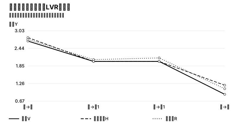
考虑四条路径：$1\to1.4\to1.8$、$1\to1.4\to1$、$1\to0.6\to1$、$1\to0.6\to0.2$。这是参考论文有限树的教学重建：每个节点上下各半的模型概率，使价格为鞅；不是对未来币价的预测。原文正文的最后节点与图有出入，这里采用Figure 3的0.2，并按自融资关系重新算库存。[^tree33]

再平衡基准始终把X库存调到池子的 $x^*(P)$，但每次都按变化后的参考价交易。若第 $k$ 次价格为 $P_k$，则

$$
\begin{aligned}
x_k&=1/\sqrt{P_k},\\
y_k^{R}&=y_{k-1}^{R}-P_k(x_k-x_{k-1}),\\
R_k&=P_kx_k+y_k^{R}.
\end{aligned}
$$

第二式是自融资条件：买X减少Y，卖X增加Y，没有外部注资。注意它的 $y_k^R$ 不必等于池子的 $\sqrt{P_k}$。

我们慢慢走一次上涨后回归的路径。价格到1.4时，基准卖出 $1-1/\sqrt{1.4}=0.154846$ X，按1.4收到0.216784 Y，因此 $y_1^R=1.216784$。此刻总财富2.4，而池子只有 $2\sqrt{1.4}=2.366432$。两者持有相同0.845154 X，差别全在Y。

下一步价格回到1，基准买回0.154846 X，支出0.154846 Y，剩1.061938 Y。加上1X，财富2.061938。池子回到1X+1Y，财富2。它相对原封不动的持币没有亏损，却比同库存再平衡基准少0.061938。

<figure class="pfh-responsive-figure"><div class="svg-wide"><img src="/notebook/labs/p-ijklm/figures/P33-a.svg" alt="四条价格路径上，池子、静态持币与自融资再平衡的终值。相同终价并不产生相同LVR。"></div><div class="svg-narrow pfh-native"><p class="pfh-figure-title">同终价的两条路径，LVR仍不同</p><p class="pfh-figure-note">无手续费与成本；四路径是模型状态，不是时间</p><ul class="pfh-legend"><li><svg viewBox="0 0 32 12" width="32" height="12" aria-hidden="true"><path d="M1 6H31" stroke="currentColor" stroke-width="3" stroke-dasharray=""/></svg><span>池子V</span></li><li><svg viewBox="0 0 32 12" width="32" height="12" aria-hidden="true"><path d="M1 6H31" stroke="currentColor" stroke-width="3" stroke-dasharray="10 5"/></svg><span>静态持币H</span></li><li><svg viewBox="0 0 32 12" width="32" height="12" aria-hidden="true"><path d="M1 6H31" stroke="currentColor" stroke-width="3" stroke-dasharray="2 5"/></svg><span>再平衡R</span></li></ul><p class="pfh-axis-label">财富Y</p><div class="pfh-plot" style="--pfh-y-label-ch:5"><div class="pfh-y-ticks"><span style="top:100.0%">0.67</span><span style="top:75.0%">1.26</span><span style="top:50.0%">1.85</span><span style="top:25.00000000000001%">2.44</span><span style="top:0.0%">3.03</span></div><svg class="pfh-plot-svg" viewBox="95.0 105.0 670.0 240.0" preserveAspectRatio="none" aria-hidden="true"><line class="grid" x1="95" y1="345.0" x2="765" y2="345.0" vector-effect="non-scaling-stroke"/><line class="grid" x1="95" y1="285.0" x2="765" y2="285.0" vector-effect="non-scaling-stroke"/><line class="grid" x1="95" y1="225.0" x2="765" y2="225.0" vector-effect="non-scaling-stroke"/><line class="grid" x1="95" y1="165.00000000000003" x2="765" y2="165.00000000000003" vector-effect="non-scaling-stroke"/><line class="grid" x1="95" y1="105.0" x2="765" y2="105.0" vector-effect="non-scaling-stroke"/><polyline points="95.00,140.08 318.33,209.48 541.67,209.48 765.00,321.77" fill="none" stroke="currentColor" stroke-width="2.7" stroke-dasharray="" vector-effect="non-scaling-stroke"/><polyline points="95.00,128.23 318.33,209.48 541.67,209.48 765.00,290.74" fill="none" stroke="currentColor" stroke-width="2" stroke-dasharray="10 5" vector-effect="non-scaling-stroke"/><polyline points="95.00,134.52 318.33,203.19 541.67,197.66 765.00,302.56" fill="none" stroke="currentColor" stroke-width="2" stroke-dasharray="2 5" vector-effect="non-scaling-stroke"/><circle cx="95.0" cy="140.08085769062882" r="3.5" fill="white" stroke="currentColor" vector-effect="non-scaling-stroke"/><circle cx="318.33333333333337" cy="209.48153645894246" r="3.5" fill="white" stroke="currentColor" vector-effect="non-scaling-stroke"/><circle cx="541.6666666666667" cy="209.48153645894246" r="3.5" fill="white" stroke="currentColor" vector-effect="non-scaling-stroke"/><circle cx="765.0" cy="321.7741935483871" r="3.5" fill="white" stroke="currentColor" vector-effect="non-scaling-stroke"/><circle cx="95.0" cy="128.2258064516129" r="3.5" fill="white" stroke="currentColor" vector-effect="non-scaling-stroke"/><circle cx="318.33333333333337" cy="209.48153645894246" r="3.5" fill="white" stroke="currentColor" vector-effect="non-scaling-stroke"/><circle cx="541.6666666666667" cy="209.48153645894246" r="3.5" fill="white" stroke="currentColor" vector-effect="non-scaling-stroke"/><circle cx="765.0" cy="290.737266466272" r="3.5" fill="white" stroke="currentColor" vector-effect="non-scaling-stroke"/><circle cx="95.0" cy="134.51685848689462" r="3.5" fill="white" stroke="currentColor" vector-effect="non-scaling-stroke"/><circle cx="318.33333333333337" cy="203.19048442366073" r="3.5" fill="white" stroke="currentColor" vector-effect="non-scaling-stroke"/><circle cx="541.6666666666667" cy="197.65905327888825" r="3.5" fill="white" stroke="currentColor" vector-effect="non-scaling-stroke"/><circle cx="765.0" cy="302.5597496463261" r="3.5" fill="white" stroke="currentColor" vector-effect="non-scaling-stroke"/></svg><div class="pfh-x-ticks"><span class="first" style="left:0.0%">上→上</span><span class="" style="left:33.333333333333336%">上→回1</span><span class="" style="left:66.66666666666667%">下→回1</span><span class="last" style="left:100.0%">下→下</span></div></div></div></figure>

<a id="p33-lvr"></a>
## 3. LVR不是相对持币损失的新名字

这里定义无费的 $\mathrm{LVR}_k=R_k-V(P_k)$。它比较的是同风险库存基准与池子，不是直接比较静态持币。

| 价格路径 | 池子V，Y | 静态持币H，Y | 再平衡R，Y | LVR=R−V，Y |
|---|---:|---:|---:|---:|
| 1→1.4→1.8 | 2.683282 | 2.800000 | 2.738062 | 0.054780 |
| 1→1.4→1 | 2.000000 | 2.000000 | 2.061938 | 0.061938 |
| 1→0.6→1 | 2.000000 | 2.000000 | 2.116398 | 0.116398 |
| 1→0.6→0.2 | 0.894427 | 1.200000 | 1.083602 | 0.189175 |

两条回到1的路径，$V-H$ 都为零，LVR却不同。这不是两个损失指标互相矛盾，而是它们问了不同的问题：前者问“比一直拿着初始资产怎样”，后者问“同样改变风险库存，但在参考价交易，会怎样”。

还有一个直接的数学检查。因为 $V'(P)=x^*(P)$ 且 $V$ 凹，单步有

$$V(P_k)-V(P_{k-1})\le x^*(P_{k-1})(P_k-P_{k-1}).$$

右边恰是再平衡基准在价格变化、尚未调仓前的财富增量。于是每一步 $R-V$ 的增量非负。证明只用正价、凹函数切线不等式及自融资，不需要读者先学随机微积分。

在这棵模型Q树上，基准与持币的期望均为2Y，池子期望1.894427Y，所以期望无费LVR为0.105573Y。这个Q期望用于检查模型的公平参考交易，不是现实LP预期收益。现实的参考市场也有成本，不能把理想基准的收益直接当作可实施套利。

<a id="p33-fees"></a>
## 4. 手续费另放一层，不能悄悄改掉基准

前面的V与R都是无费库存财富。现在独立假设池子另收0.02Y费用、支出0.005Y成本，费用提取到池外现金，不再投入库存。净费用现金为0.015Y，总净所得为

$$W_{\rm LP}=V+0.02-0.005=V+0.015.$$

四条路径的无费库存和结构LVR并未改变，只是总所得多了0.015Y。期望净所得变成1.909427Y，与R的期望差变成0.090573Y；这个含费差额不能重新叫作刚才定义的结构LVR，也不能直接继承它每步非负的结论。若某段费用较高，净差额完全可能减小甚至反号。

这种单列费用的处理对应论文的简化假设：费用用计价资产支付，不改变池子曲线。[^fee33] 真实协议是否把费用再投入、怎样分配，以及调整头寸要付多少成本，需要另读具体协议和实际记录，而不是给V多加一个“年化APR”。

<a id="p33-range"></a>
## 5. 集中区间：价格越界以后，你拿着什么

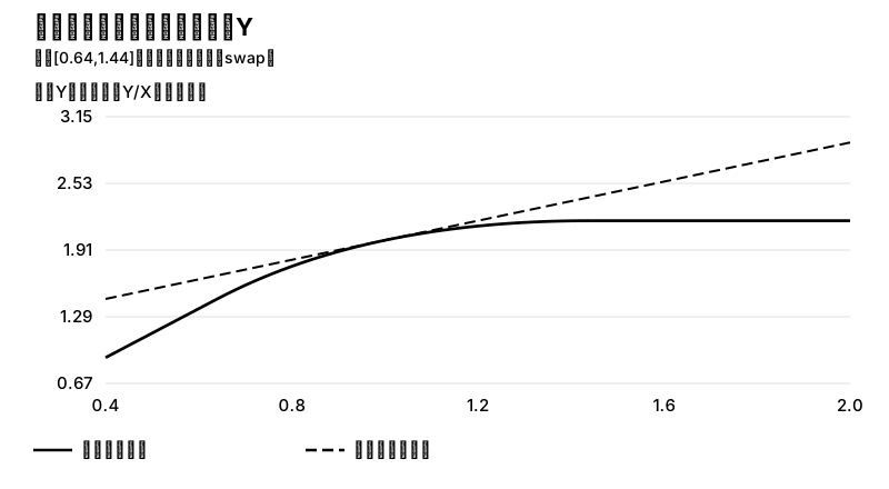
Uniswap v3的集中流动性允许把流动性放在有限区间。价格越过区间后，头寸变为单一资产、不再提供该区间内的活跃交换流动性；重新进入时才重新活跃。[^uni33]

我们用连续价格近似，区间 $[p_a,p_b]=[0.64,1.44]$，起点P=1，初值2Y。区间内的实际库存为

$$
\begin{aligned}
x(P)&=L\left(\frac1{\sqrt P}-\frac1{\sqrt{p_b}}\right),\\
y(P)&=L\left(\sqrt P-\sqrt{p_a}\right).
\end{aligned}
$$

在P=1时，$x=L/6$、$y=L/5$，因此初值 $x+y=11L/30=2$，解得 $L=60/11$，$x_0=10/11$ X、$y_0=12/11$ Y。

若价格涨到1.69，已经超过上界。头寸变成 $x=0$、$y=L(\sqrt{1.44}-\sqrt{0.64})=24/11$ Y，总库存价值2.181818Y。它卖完了X，不再跟随X继续上涨。相同初始库存的静态持币此时是

$$H=1.69\times\frac{10}{11}+\frac{12}{11}=2.627273\text{ Y}.$$

<figure class="pfh-responsive-figure"><div class="svg-wide"><img src="/notebook/labs/p-ijklm/figures/P33-b.svg" alt="集中区间内外的X、Y库存及活跃状态。上穿区间后X库存归零，并不是资金消失。"></div><div class="svg-narrow pfh-native"><p class="pfh-figure-title">集中区间：上界以后库存全为Y</p><p class="pfh-figure-note">区间[0.64,1.44]；越界不再收取新的swap费</p><ul class="pfh-legend"><li><svg viewBox="0 0 32 12" width="32" height="12" aria-hidden="true"><path d="M1 6H31" stroke="currentColor" stroke-width="3" stroke-dasharray=""/></svg><span>区间库存市值</span></li><li><svg viewBox="0 0 32 12" width="32" height="12" aria-hidden="true"><path d="M1 6H31" stroke="currentColor" stroke-width="3" stroke-dasharray="10 5"/></svg><span>原库存持币市值</span></li></ul><p class="pfh-axis-label">财富Y；横轴价格Y/X；费用另列</p><div class="pfh-plot" style="--pfh-y-label-ch:5"><div class="pfh-y-ticks"><span style="top:100.0%">0.67</span><span style="top:75.0%">1.29</span><span style="top:50.0%">1.91</span><span style="top:25.0%">2.53</span><span style="top:0.0%">3.15</span></div><svg class="pfh-plot-svg" viewBox="95.0 105.0 670.0 240.0" preserveAspectRatio="none" aria-hidden="true"><line class="grid" x1="95" y1="345.0" x2="765" y2="345.0" vector-effect="non-scaling-stroke"/><line class="grid" x1="95" y1="285.0" x2="765" y2="285.0" vector-effect="non-scaling-stroke"/><line class="grid" x1="95" y1="225.0" x2="765" y2="225.0" vector-effect="non-scaling-stroke"/><line class="grid" x1="95" y1="165.0" x2="765" y2="165.0" vector-effect="non-scaling-stroke"/><line class="grid" x1="95" y1="105.0" x2="765" y2="105.0" vector-effect="non-scaling-stroke"/><polyline points="95.00,321.77 103.38,317.38 111.75,312.98 120.12,308.58 128.50,304.18 136.88,299.78 145.25,295.38 153.62,290.98 162.00,286.58 170.38,282.18 178.75,277.79 187.12,273.39 195.50,268.99 203.88,264.69 212.25,260.59 220.62,256.68 229.00,252.95 237.38,249.39 245.75,245.99 254.12,242.76 262.50,239.68 270.88,236.75 279.25,233.96 287.62,231.30 296.00,228.78 304.38,226.39 312.75,224.12 321.12,221.97 329.50,219.94 337.88,218.02 346.25,216.20 354.62,214.50 363.00,212.89 371.38,211.39 379.75,209.98 388.12,208.66 396.50,207.44 404.88,206.31 413.25,205.26 421.62,204.30 430.00,203.42 438.38,202.62 446.75,201.89 455.12,201.25 463.50,200.68 471.88,200.18 480.25,199.76 488.62,199.40 497.00,199.11 505.38,198.89 513.75,198.73 522.12,198.64 530.50,198.61 538.88,198.61 547.25,198.61 555.62,198.61 564.00,198.61 572.38,198.61 580.75,198.61 589.12,198.61 597.50,198.61 605.88,198.61 614.25,198.61 622.62,198.61 631.00,198.61 639.38,198.61 647.75,198.61 656.12,198.61 664.50,198.61 672.88,198.61 681.25,198.61 689.62,198.61 698.00,198.61 706.38,198.61 714.75,198.61 723.12,198.61 731.50,198.61 739.88,198.61 748.25,198.61 756.62,198.61 765.00,198.61" fill="none" stroke="currentColor" stroke-width="2.7" stroke-dasharray="" vector-effect="non-scaling-stroke"/><polyline points="95.00,268.99 103.38,267.23 111.75,265.47 120.12,263.71 128.50,261.95 136.88,260.19 145.25,258.43 153.62,256.67 162.00,254.91 170.38,253.15 178.75,251.39 187.12,249.63 195.50,247.87 203.88,246.11 212.25,244.35 220.62,242.60 229.00,240.84 237.38,239.08 245.75,237.32 254.12,235.56 262.50,233.80 270.88,232.04 279.25,230.28 287.62,228.52 296.00,226.76 304.38,225.00 312.75,223.24 321.12,221.48 329.50,219.72 337.88,217.96 346.25,216.20 354.62,214.44 363.00,212.68 371.38,210.92 379.75,209.16 388.12,207.40 396.50,205.65 404.88,203.89 413.25,202.13 421.62,200.37 430.00,198.61 438.38,196.85 446.75,195.09 455.12,193.33 463.50,191.57 471.88,189.81 480.25,188.05 488.62,186.29 497.00,184.53 505.38,182.77 513.75,181.01 522.12,179.25 530.50,177.49 538.88,175.73 547.25,173.97 555.62,172.21 564.00,170.45 572.38,168.70 580.75,166.94 589.12,165.18 597.50,163.42 605.88,161.66 614.25,159.90 622.62,158.14 631.00,156.38 639.38,154.62 647.75,152.86 656.12,151.10 664.50,149.34 672.88,147.58 681.25,145.82 689.62,144.06 698.00,142.30 706.38,140.54 714.75,138.78 723.12,137.02 731.50,135.26 739.88,133.50 748.25,131.74 756.62,129.99 765.00,128.23" fill="none" stroke="currentColor" stroke-width="2" stroke-dasharray="10 5" vector-effect="non-scaling-stroke"/></svg><div class="pfh-x-ticks"><span class="first" style="left:0.0%">0.4</span><span class="" style="left:50.0%">1.2</span><span class="last" style="left:100.0%">2.0</span></div></div></div></figure>

本分支另设累计费用0.05Y、成本0.01Y，净所得2.221818Y。这里绝不沿用上一节的0.02／0.005；两组是不同教学分支。若要追平此路径上的静态持币，需要累计费用

$$H-V+\mathrm{cost}=2.627273-2.181818+0.01=0.455455\text{ Y}.$$

这只是给定路径的门槛，不是交易量会产生该费用的预测。区间外也不能继续拿此前费率乘时间。若主动移区间，需要新交易、资产转换及gas；这些改变原有策略，应作为新决策记录。本例没有声称这两个边界是某个已部署池的有效tick。

<a id="p33-theory"></a>
## 6. 选读：连续时间里同一个差额

主线有限树已经足以理解库存和基准。熟悉Itô公式的读者可以再把它连到连续形式。在零利率、正的连续价格过程、固定池子曲线、$V\in C^2$、$V'=x^*$，以及使随机积分成立的局部平方可积条件下，自融资基准为

$$R_t=V(P_0)+\int_0^t x^*(P_s)\,dP_s.$$

对V用Itô公式并相减，完整得到

$$R_t-V(P_t)=-\frac12\int_0^t V''(P_s)\,d[P]_s.$$

凹性令被积量非负。若 $d[P]_t=\sigma_t^2P_t^2dt$，瞬时增长率就是 $\tfrac12\sigma_t^2P_t^2|x^{*\prime}(P_t)|$。若还要把R称为期望保持不变的Q鞅，需要相应真鞅/可积条件，不能仅凭形式随机积分就跳到期望等式。[^proof33]

这段推导属于连续、无摩擦参考市场模型。跳跃价格、离散成交、费用改变曲线或主动增减流动性时，必须重新检查条件，不能原样贴上“保证净盈利”或“永远亏损”的结论。

<a id="p33-lab"></a>
## 7. 实验、自测与完整解析

<div data-experiment-slot="EXP-P33-LP"></div>

先不勾选费用，比较两条回到P=1的路径，逐行检查再平衡现金。接着启用0.015Y净费用层，观察总所得变化而结构LVR不变。最后切换集中区间，移动终点价格跨过上界，确认X变为0，以及费用参数切换为独立0.05／0.01。

**解释题。** 为什么1→1.4→1与1→0.6→1的相对静态持币差均为零，而LVR分别为0.061938和0.116398？

静态持币只保留初始1X+1Y，回到同一终价便回到同一财富。再平衡基准在上行路径先卖后买，在下行路径先买后卖；两条路径的交易数量不同，因此留下不同Y余额。LP虽然回到初始库存，却没有取得按参考价逐次交易的那份现金。

**迁移题。** 若有限树净费用提高到0.12Y，是否应该把所有原LVR减0.12并继续叫它“非负LVR”？

不应该。结构LVR仍由无费R−V定义。变化的是总净所得V+0.12及其相对R的净差额；部分路径此差额会变负，并不违反无费凹性结论。名称和比较对象不能随显示方便而更换。

**区间题。** 越过上界后还能用此前每日期望手续费继续累计收入吗？

不能。头寸已不活跃，直到重新进入区间才重新参与交换。即便在区间内，手续费也依赖真实交易流量和所占流动性，而非已知固定息票。恢复活跃的主动移仓又有新的成本与风险。

**完成标准。** 能用单位一致的库存与现金账同时重建LP、HODL和再平衡基准，分清无费LVR、费用层和区间层，再讨论实际收益，而不是先把一个APR当成投资结论。

[^lvr33]: Milionis、Moallemi、Roughgarden、Zhang，[Automated Market Making and Loss-Versus-Rebalancing](https://arxiv.org/pdf/2208.06046v6)，固定v6，2026-08-20上传，§2–3及§4的价值/自融资定义。本文推演的是透明模型，不采用未读取的§7实证比例。
[^tree33]: 同文§5.1与Figure 3。正文DD=0.4与图DD=0.2不一致；采用明确的0.2树以保持各节点模型Q鞅，并自行重建Panel C库存，不照抄不一致的终点数。
[^fee33]: 同文§3“Noise traders”及§5.1；费用独立于库存曲线的假设与无费树分开。
[^uni33]: Adams等，[Uniswap v3 Core](https://app.uniswap.org/whitepaper-v3.pdf)，2021-03，§2、§2.1及§3.1–3.2，采用实际库存、出区间与费用独立记账，不采用旧费率列表作为当前完整产品目录。
[^proof33]: LVR v6 §4 Assumption 1、Lemmas 1–2、自融资定义及Appendix A.1/A.2。连续形式需要相应光滑与可积条件；本篇有限树无需Itô作为先修。

<script src="/notebook/labs/p-ijklm/reader-adapter.js" defer></script>


## Experiment inputs and static equivalents
```json
[
  {
    "id": "EXP-P33-LP",
    "node_id": "P33",
    "title": "流动性提供：库存、费用与比较基准",
    "anchor": "p33-lab",
    "description": "重建LP、持币和自融资基准，分离结构LVR、费用层与集中区间状态。",
    "inputs": {
      "frozen_ids": [
        "SIM-PM-LVR-TREE-01"
      ],
      "operational_keys": [],
      "units": "逐字段以shared/final-shared-inputs.json与operational-inputs.json为准"
    },
    "outputs": {
      "default_location": "agent_packet.supplied_inputs.static_default_result"
    },
    "algorithm": "https://ou-liu-red-sugar.github.io/notebook/labs/p-ijklm/engine.js; P26 consumes QT24 outputs without rerunning simulation.",
    "views": [
      "LP/HODL/再平衡基准",
      "集中区间库存和独立费用"
    ],
    "boundaries": [
      "真实规格不等于当前保证金或成交",
      "不得从终点补造未提供的资金路径",
      "输入无效即停止，不能沿用旧结果"
    ],
    "static_equivalent": {
      "figures": [
        "https://ou-liu-red-sugar.github.io/notebook/labs/p-ijklm/figures/P33-a.svg",
        "https://ou-liu-red-sugar.github.io/notebook/labs/p-ijklm/figures/P33-b.svg"
      ],
      "body_tables": true,
      "event_data": [
        {
          "path": "https://ou-liu-red-sugar.github.io/notebook/labs/p-ijklm/shared/lp-self-financing-ledgers.csv",
          "branch": "core",
          "sha256": "e1cd072b8005a5be59031fbdfc0e08750c91753e1e462cf8b5cb6cb12c452ac8",
          "format": "csv",
          "public_access": "随本ZIP及复制教学包提供的UTF-8附件；非内部盘符"
        },
        {
          "path": "https://ou-liu-red-sugar.github.io/notebook/labs/p-ijklm/shared/lp-range-grid.csv",
          "branch": "core",
          "sha256": "62c729e58b368e35d526356452474ec81ecad64ac45aaea8b81a9974b73e5a66",
          "format": "csv",
          "public_access": "随本ZIP及复制教学包提供的UTF-8附件；非内部盘符"
        }
      ]
    },
    "input_controls": [
      {
        "key": "mode",
        "label": "比较对象",
        "type": "select",
        "default": "finite",
        "options": [
          {
            "value": "finite",
            "label": "无费树与独立费用层"
          },
          {
            "value": "range",
            "label": "集中区间独立分支"
          }
        ]
      },
      {
        "key": "path",
        "label": "有限树路径",
        "type": "selectnum",
        "default": 1,
        "options": [
          {
            "value": 1,
            "label": "1→1.4→1"
          },
          {
            "value": 0,
            "label": "1→1.4→1.8"
          },
          {
            "value": 2,
            "label": "1→0.6→1"
          },
          {
            "value": 3,
            "label": "1→0.6→0.2"
          }
        ]
      },
      {
        "key": "fee",
        "label": "有限树加0.02费、减0.005成本",
        "type": "check",
        "default": false
      },
      {
        "key": "price",
        "label": "区间终点P（Y/X）",
        "type": "number",
        "default": 1.69
      }
    ],
    "input_uri": "https://ou-liu-red-sugar.github.io/notebook/labs/p-ijklm/shared/final-shared-inputs.json"
  }
]
```

## Sources
- [Automated Market Making and Loss-Versus-Rebalancing](https://arxiv.org/pdf/2208.06046v6): 无费库存、同风险库存的自融资基准、结构LVR与独立费用层。
- [Uniswap v3 Core](https://app.uniswap.org/whitepaper-v3.pdf): 集中区间的真实/虚拟储备与有限交换；手续费增长公式以固定代码作局部单位校正。

本批读取范围：集中区间实际库存、出区间状态与费用独立记账。

## Content relations
```json
[
  {
    "from": "zh-p33",
    "relation": "part_of",
    "to": "portfolio-implementation",
    "reason": "主要 topic 归属"
  },
  {
    "from": "zh-p33",
    "relation": "uses_method",
    "to": "zh-p02",
    "reason": "调用局部概念；本篇同时给出完成算例所需的最小说明。"
  },
  {
    "from": "zh-p33",
    "relation": "illustrated_by",
    "to": "p33-rebalancing",
    "reason": "同一冻结对象和明确身份的算例。"
  },
  {
    "from": "p33-rebalancing",
    "relation": "supported_by",
    "to": "MOD-LVR",
    "reason": "无费库存、同风险库存的自融资基准、结构LVR与独立费用层。",
    "locator": "§3资产/费用设置；§4自融资定义；§5.1完整有限树与Figure3；使用本文给出的凹性推导",
    "scope": "无费库存、同风险库存的自融资基准、结构LVR与独立费用层。"
  },
  {
    "from": "p33-range",
    "relation": "supported_by",
    "to": "MOD-UNISWAP-V3",
    "reason": "集中区间实际库存、出区间状态与费用独立记账。",
    "locator": "PDFpp1–3；§2/2.1与§3.1–3.2",
    "scope": "集中区间实际库存、出区间状态与费用独立记账。"
  },
  {
    "from": "p33-theory",
    "relation": "supported_by",
    "to": "MOD-LVR",
    "reason": "选择连续时间推导时；§4及AppendixA.1/A.2",
    "locator": "§4 Assumption1、Lemmas1–2及AppendixA.1/A.2完整相关证明",
    "scope": "选择连续时间推导时；§4及AppendixA.1/A.2",
    "branch": "continuous"
  },
  {
    "from": "p33-lab",
    "relation": "illustrated_by",
    "to": "EXP-P33-LP",
    "reason": "重建LP、持币和自融资基准，分离结构LVR、费用层与集中区间状态。"
  }
]
```

## Related entries